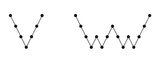
The classic iterative method essentially only plays a "smooth" effect, even if it can quickly eliminate the high-frequency part of the residual, but the effect is not very good for the low-frequency part. The basic idea of the multi-grid method is: first of all Establish a set of coarse and fine grids for the fixed solution area, and form the corresponding difference or finite element discrete equation. For this discrete equation, first use the usual iterative method on the fine grid, such as Richardson iteration and Gauss-Seidel iteration. Iteratively eliminate the high-frequency part of the residual, and then transfer the low-frequency part of the residual to the coarse grid for correction. After several cycles, a solution that satisfies the accuracy is obtained. Since the residual correction is performed on the coarse grid , So the corresponding workload is relatively small.
The Jacobi and Gauss-Seidel iterations produce smooth errors. The error vector $e$ has its high frequencies nearly removed in a few iterations. But low frequencies are reduced very slowly. Convergence requires $O(N^2)$ iterations - which can be unacceptable. The extremely effective multigrid idea is to change to a coarser grid, on which "smooth becomes rough" and low frequencies act like higher frequencies.
On that coarser grid a big piece of the error is removable. We iterate only a few times before changing from fine to coarse and coarse to fine. The remarkable result is that multigrid can solve many sparse and realistic systems to high accuracy in a fixed number of iterations, not growing with $n$.
Multigrid is especially successful for symmetric systems. The key new ingredients are the (rectangular !) matrices $R$ and $I$ that change grids:
-
A restriction matrix R transfers vectors from the fine grid to the coarse grid
-
An interpolation matrix $I=I_{2h}^h$ returns to the fine grid
-
The original matrix $A_h$ on the fine grid is approximated by $A_{2h}=RA_HI$ on the coarse grid. This $A_{2h}$ is smaller and easier and faster than $A_h$. I will start with interpolation (a 7 by 3matrix $I$ that takes 3 v's to 7 u's):
$$
\frac{1}{2}\left[\begin{matrix}1&&\\2&&\\1&1&\\&2&\\&1&1\\&&2\\&&1\end{matrix}\right]\left[\begin{matrix}v_1\\v_2\\v_3\end{matrix}\right]=\left[\begin{matrix}v_1/2\\v_1\\v_1/2+v_2/2\\v_2\\v_2/2+v_3/2\\v_3\\v_3/2\end{matrix}\right]=\left[\begin{matrix}u_1\\u_2\\u_3\\u_4\\u_5\\u_6\\u_7\end{matrix}\right]
$$
Interpolation $Iv=u$, $u$ on the fine $(h)$ grid, $v$ on the coarse $(2h)$ grid.
The second matrix we need is a restriction matrix $R_h^{2h}$. It transfers $u$ on a fine grid to $v$ on a coarse grid. One possibility is the one-zero "injection matrix" that simply copies $v$ from grid values $u_{2j+1}$. Another possibility (which we adopt) is the full weighting operator R that comes from transposing $I_{2h}^h$.
Fine grid $h$ to coarse grid $2h$ by a restriction matrix $R=\frac{1}{2}I^T$
$$
\frac{1}{4}\left[\begin{matrix}1&2&1&&&&\\&&1&2&1&&\\&&&&1&2&1\end{matrix}\right]\left[\begin{matrix}u_1\\u_2\\u_3\\u_4\\u_5\\u_6\\u_7\end{matrix}\right]=\left[\begin{matrix}v_1\\v_2\\v_3\end{matrix}\right]
$$
Geometric multigrid, GMG
Get the iterative result from the original mesh $x_1$, and we require equations satisfied
$$
A_1\vec{e_1}=\vec{r_1}=\vec{b}-A\vec{x_1}
$$
Equivalent in coarse grid to solve
$$
A_1\vec{e_2}=\vec{r_2}
$$
Among them, $\vec{r_2}$ is obtained by down sampling from $\vec{r_1}$ which is equivalent to the left multiplication matrix
$$
C_{12}=\left[\begin{matrix}\ddots&\ddots&\ddots&&&&&&&&\\&&w_{c_1}&w_{c_0}&w_{c_1}&&&&&&\\&&&&w_{c_1}&w_{c_0}&w_{c_1}&&&&\\&&&&&&w_{c_1}&w_{c_0}&w_{c_1}&&\\&&&&&&&&\ddots&\ddots&\ddots\end{matrix}\right]
$$
After solving the $\vec{e_2}$ in which the low-frequency error is suppressed, the $\vec{e_1}$ is obtained by interpolation, and the $\vec{x_1}+\vec{e_1}$ is used as the new solution.
Interpolation is equivalent to left multiplication matrix
$$
I_{21}=\left[\begin{matrix}\ddots&&&\\\ddots&&&\\\ddots&w_{i_1}&&\\&w_{i_0}&&\\&w_{i_1}&w_{i_1}&\\&&w_{i_0}&\\&&w_{i_1}&\\&&&\ddots\\&&&\ddots\\&&&\ddots\end{matrix}\right].
$$
Sampling the residual to a coarse grid, and interpolate the solution to a fine grid after solving, that is $\vec{r_2}=C_{12}\vec{r_1}$, $\vec{e_1}=I_{21}\vec{e_2}$.
Comparison available $A_2=C_{12}A_1I_{21}$,
Multigrid algorithm solution $A_1\vec{x}=\vec{b}$,
- If the grid size is small enough to solve the equation accurately or imprecisely, return the solution;.
- Otherwise ,Solve iteratively with $\vec{x_0}=0$ as the initial iterative step, obtain $\vec{x_1}$. And calculate residual $\vec{r_1}=A_1\vec{x_1}$.
- Coarse the residuals $\vec{r_2}=C_{12}\vec{r_1}$.
- order $A_2=C_{12}A_1I_{21}$, Solve $A_2\vec{e_2}=\vec{r}$ using multi-grid algorithm.
- Interpolate the solution and accumulate $\vec{x_2}=\vec{x_1}+I_{21}\vec{e_2}$.
- Iterate with $\vec{x_2}$ as the initial iterative step to obtain $\vec{x_3}$.


0 条评论